Optimizing Image Processing on the Edge
Webassembly is the primary target. It is independent of processor architecture, which is useful because many of Scailable's customers run esoteric hardware/OS combinations. If the specific hardware is known in advance, particularly expensive operations can be run natively on either the CPU or GPU. Furthermore webassembly is evaluated in a sandbox providing much better security and isolation than executing raw machine code that is sent over the wire (though security is still a concern).
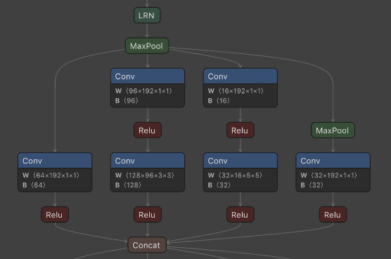
The neural networks are provided by machine learning experts in the ONNX format. ONNX represents a neural network as a graph of data flow and computation nodes. It is a compact representation, but is just a specification of the computation, on an abstract level.
To apply the network to real data, the ONNX specification needs to be converted into code: the computation nodes are turned into runnable functions, and these functions must be called in the right order to replicate the structure of the ONNX graph.
The subject of this article is the resize node. Intuitively, the resize node either stretches or compresses an image. When an image is stretched, we end up with more pixels than we had, but what color should these new pixels have?
Profiling showed that the resize node type was particularly slow. We set out to write a faster implementation.
Linear interpolation
The simplest method for picking the new pixel values is linear interpolation. In a black and white image, each pixel has a color value between 0.0 (black) and 1.0 (white). With linear interpolation, we pick evenly spaced points between two values. For instance, given two pixels
0.0 | 1.0
Scaling by a factor 1.5 gives an image with 3 pixels:
0.0 | 0.5 | 1.0
And scaling by a factor of 2 yields an image with 4 pixels:
0.0 | 0.33 | 0.66 | 1.0 |
For RGB images the method is the same, it just has to be repeated for each of the three color channels.
While simple to understand and compute, linear interpolation only considers either the row or the column. For an actual image, that would give a weird result. For improved results we need to consider more neighbors.
Bilinear interpolation
With bilinear interpolation we consider the neighbor to the left, right, top and bottom. Linear interpolation in 2D (i.e. bilinear) can be seen as 2 1D (i.e. linear) interpolations: first along one axis, then along the other. Say we want to scale this matrix in both dimensions with a factor 1.5:
1 3
5 7
We could then first interpolate the row
1 2 3
5 6 7
And then the column
1 2 3
3 4 4
5 6 7
This approach is valid and correct, but inefficient in practice because an intermediate array is constructed. A more efficient approach is to loop over the output matrix, and for each position find out what its final value is by looking up the necessary values in the input. This approach uses the minimal amount of memory, and can be implemented without recursion.
Other interpolation modes
The ONNX resize operator has 2 other interpolation modes: nearest and cubic. Nearest is simple: for any point in the output it picks the closest point in the input and uses its value. Cubic however is more complex because it uses more input points. The result is a smoother image, at the cost of increased computation time.
Process
We implemented all 3 interpolation modes for up to 3 dimensions, which covers the vast majority of uses in the wild. For higher dimensions and edge cases we use a much slower fallback. We can always optimize edge cases further if required.
The algorithm is implemented in C and compiled to webassembly. Web assembly is inherently slower than running machine code, but has advantages in distribution: it runs on any processor architecture and operating system.
Let's look briefly at 2D linear interpolation, just to get an idea of roughly what this code does.
void bilinear_interpolation(float *data, uint32_t input_width,
                            uint32_t input_height, uint32_t output_width,
                            uint32_t output_height, float *output) {
The data is passed in as one contiguous array of floats. The input width and height determine the rows and columns.
First we need to know our scaling factors.
    float x_ratio, y_ratio;

    if (output_width > 1) {
        x_ratio = ((float)input_width - 1.0) / ((float)output_width - 1.0);
    } else {
        x_ratio = 0;
    }

    if (output_height > 1) {
        y_ratio = ((float)input_height - 1.0) / ((float)output_height - 1.0);
    } else {
        y_ratio = 0;
    }
And then we walk over each pixel in the output and determine its value:
    for (int i = 0; i < output_height; i++) {
        for (int j = 0; j < output_width; j++) {
            float x_l = floor(x_ratio * (float)j);
            float y_l = floor(y_ratio * (float)i);
            float x_h = ceil(x_ratio * (float)j);
            float y_h = ceil(y_ratio * (float)i);

            float x_weight = (x_ratio * (float)j) - x_l;
            float y_weight = (y_ratio * (float)i) - y_l;

            float a = data[(int)y_l * input_width + (int)x_l];
            float b = data[(int)y_l * input_width + (int)x_h];
            float c = data[(int)y_h * input_width + (int)x_l];
            float d = data[(int)y_h * input_width + (int)x_h];

            float pixel = a * (1.0 - x_weight) * (1.0 - y_weight) +
                          b * x_weight * (1.0 - y_weight) +
                          c * y_weight * (1.0 - x_weight) +
                          d * x_weight * y_weight;

            output[i * output_width + j] = pixel;
        }
    }
}
First, we find the indices of the four surrounding points (left, down, right, up). Then we determine the weight for each axis, i.e. the ratio between the low and high point. Next, we load the values of the surrounding points, and use a series of linear interpolations to get the value for the current pixel.
If you have suggestions to speed this up even further (using C99) please let us know. The full code is here.
Results
We have observed 1000X speedups on real inputs. Big factors here are the reduction in stack frames (as we have no recursion) and more predictable memory access.
I think that given the constraints of webassembly, this is close to the best we can do. Wasm does not have dedicated SIMD instructions, and we can't offload work to the GPU. What we can still explore is exposing C functions to the webassembly environment. These C functions can use vectorizing instructions or GPU hardware if available. We have seen good results with this approach for other operators.
Another avenue of research is combining and fusing computation stages. Here is an excellent talk on the challenges of organizing a tensor processing task, link. It would be interesting to see what kind of impact these techniques could have.
We look forward to working on more of these challenging optimizations with Scailable. If you have questions of suggestions, feel free to contact me at folkert@tweedegolf.com.